4.4 Short-range extrapolation
LEARNING OBJECTIVES:
|
Compare short-range extrapolation techniques for the movement of
frontal systems and associated weather.
|
The purpose of this section is to outline several methods that are
particularly suited to preparing forecasts for periods of 6 hours or less. The
techniques presented are based on extrapolation. Extrapolation is the estimating
of the future value of some variable based on past values. Extrapolation
is one of the most powerful short-range forecasting tools available to the
forecaster.
Nephanalysis may be defined as any form of analysis of the field of cloud
cover and/or type. Cloud observations received in synoptic codes permit only a
highly generalized description of the actual structure of the cloud systems.
Few forecasters make full use of the cloud reports plotted on their surface
charts, and often, the first consideration in nephanalysis is to survey what
cloud information is transmitted, and to make sure that everything pertinent is
plotted. For very short-range forecast, the charts at 6-, 12-, and 24-hour
intervals are apt to be insufficient for use of the extrapolation techniques
explained in this chapter. Either nephanalysis or surface charts should then be
plotted at the intermediate times from 3-hourly synoptic reports or even from
hourly sequences. An integrated system of forecasting ceiling, visibility, cloud
cover, and precipitation should be considered simultaneously, as these elements
are physically dependent upon the same synoptic processes. With present-day
satellite capabilities, it is rare that a nephanalysis would be manually
performed. Instead, the surface analysis and satellite imagery will be used
together.
For short-range forecasting, the question is often not whether there will be
any precipitation, but when will it begin or end.
This problem is well suited to extrapolation methods. For short-range
forecasting, the use of hourly nephanalyses often serve to "pickup"
new precipitation areas forming upstream in sufficient time to alert a
downstream area. Also, the thickening
and lowering of middle cloud decks generally indicate where an outbreak of
precipitation may soon occur.
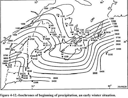
The areas of continuous, intermittent, and showery precipitation can be
outlined on a large-scale 3-hourly or hourly synoptic chart in a manner
similar to the customary shading of precipitation areas on ordinary synoptic
surface weather maps. Different types of lines, shading, or symbols can
distinguish the various types of precipitation. Isochrones of several hourly
past positions of the lines of particular interest can then be added to the
chart, and extrapolations for several hours made from them if reasonably
regular past motions are in evidence. A separate isochrone chart (or acetate
overlay) may be easier to use. Lines for the beginning of continuous
precipitation are illustrated in figure 4-12. The isochrones for showery or
intermittent precipitation usually give more uncertain and irregular patterns,
which result in less satisfactory forecasts.
When large-scale section surface weather maps are regularly drawn, it maybe
sufficient and more convenient to make all precipitation area analyses and
isochrones on these maps.
The idea of plotting observations taken at different times on a diagram
that has horizontal or vertical distance in the atmosphere as one coordinate
and time as the other has been used in various forms by forecasters for years.
The time cross section that was discussed in the AG2 TRAMAN, volume 1, unit 9,
lesson 2. is a special case of this aid, where successive information at only
one station is plotted.
One of the many obstacles the forecaster faces in preparing forecasts is the
problem of determining "when" ceilings heights will lower in areas
expecting rain. In the following paragraphs, we will discuss this dilemma.
The lowering of ceiling with continuous rain or snow in warm frontal and
upper trough situations is a familiar problem to the forecaster in many
regions. In very short-range forecasting, the question as to whether or not it
will rain or snow, and when the rain or snow will begin, is not so often the
critical question. Rather, the problem is more likely to be (assuming the rain/snow
has started) how much will the ceiling lower in 1, 2, and 3 hours, or will the
ceiling go below a certain minimum in 3 hours. The visibility in these
situations generally does not reach an operational minimum as soon as the
ceiling.
It has been shown that without sufficient convergence, advection, or
turbulence, evaporation of rain into a layer does not lead to saturation, and
causes no more than haze or light fog.
 |
It is important to recognize the difference between the behavior of the
actual cloud base height and the variation of the ceiling height, as defined
in airway reports. The ceiling usually
drops rapidly, especially during the first few hours after the rain or snow
begins. However, if the rain or snow is continuous, the true base of
the cloud layer descends gradually or steadily. The reason for this is that
below the precipitation frontal cloud layer there are usually shallow layers
in which the relative humidity is relatively high and which soon become
saturated by the rain. The cloud base itself has small, random
fluctuations in height superimposed on the general trend.
Forecasting the time when a given ceiling height will be reached during
rain is a separate problem, Nomograms, tables, air trajectories, and the time
air will become saturated can all be resolved into an objective technique
tempered with empirical knowledge and subjective considerations. This forecast
can be developed for your individual station.
The x-t diagram, as mentioned previously in this chapter, can be used to
extrapolate the trend of the ceiling height in rain.
The hourly observations should be plotted for stations near a line parallel to
the probable movement of the general rain sea, originating at your terminal
and directed toward the oncoming rain area. Ceiling-time curves for given
ceiling heights may be drawn and extrapolated. There may be systematic
geographical differences in the ceiling between stations due to local (topographic)
influences. Such differences sometimes can be anticipated from climatological
studies, or experience.
In addition, there may be a diurnal
ceiling fluctuation, which will become evident in the curve. Rapid and
erratic up-and-down fluctuations also must be dealt with. In this case, a
smoothing of the curves may be necessary before extrapolation can be made. A
slightly less accurate forecast may result from this process.
In view of the previous discussion of the precipitation ceiling problem, it is
not expected that mere extrapolation can be wholly satisfactory at a station
when the ceiling lowers rapidly during the first hours of rain, as new cloud
layers form beneath the front. However, by
following the ceiling trend at surrounding stations, patterns of abrupt
ceiling changes may be noted. These changes at nearby stations where rain
started earlier may give a clue to a likely sequence at your terminal.
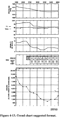
The trend chart can be a valuable forecasting tool when it is used as a
chronological portrayal of a group of related factors.
It has the added advantage of helping the forecaster to become "current"
when coming on duty. At a glance, the relieving duty forecaster is able to get
the picture of what has been occurring. Also, the forecaster is able to see the
progressive effect of the synoptic situation on the weather when the trend chart
is used in conjunction with the current surface chart.
The format of a trend chart should be a function of what is desired;
consequently, it may vary in form from situation to situation. It should,
however, contain those elements that are predictive in nature.
The trend chart is a method for graphically portaying those factors that the
forecasters generally attempt to store in their memory. Included in this trend
chart is a list of key predictor stations. The forecaster uses the hourly and
special reports from these stations as aids in making short forecasts for his/her
station. Usually, the sequences from these predictor stations are scanned and
committed to memory. The method is as follows:
-
Determine the direction from which the weather will be arriving; i.e.,
upstream.
-
Select a predictor station(s) upstream and watch for the onset of the
critical factor; for example, rain.
-
Note the effect of this factor on ceiling and visibility at predictor
station(s).
-
Extrapolate the approach of the factor to determine its onset at your
station.
-
Consider the effect of the factor at predictor station(s) in forecasting
its effect at your station.
The chief weakness of this procedure is its subjectivity. The forecaster is
required to mentally evaluate all of the information available, both for their
station and the predictor station(s).
A question posed, "How many trend charts do I need"? The answer
depends on the synoptic situation. There are times when keeping a graphic record
is unnecessary; and other times, the trend for the local station may suffice.
The trend chart format, figure 4-13, is but one suggested way of portraying the
weather record. Experimentation and improvisation are
encouraged to find the best form for any particular location or problem.
In the preceding sections of this chapter, several methods have been
described for "keeping track of the weather" on a short-term basis.
Explanations of time-distance charts, isochrone aids, trend charts, etc., have
been presented. It is usually not necessary to use all, or even most of these
aids simultaneously. The aid described in this section is designed for use in
combination with one or several of the methods previously described. Time-liners
are especially useful for isochrone analysis and follow-on extrapolation.
Inasmuch as a majority of incorrect short-range forecasts result from poor
timing of weather already upstream, an aid, such as described below, may improve
this timing.
The time-liner is simply a local area map that is covered with transparent
plastic and constructed as follows:
-
Using a large-scale map of the local area, construct a series of
concentric circles centered on your station, and equally spaced from 10 to
20 miles apart. This distance from the center to the outer circle depends
on your location, but in most cases, 100 to 150 miles is sufficient.
-
Make small numbered or lettered station circles for stations located
at varying distances and direction from your terminal. Stations likely to
experience your future weather should be selected. In addition to the
station circle indicators, significant topographical features, such as
rivers or mountains, maybe indicated on the base diagram. (Aeronautical
charts include these features.)
-
Cover and bind the map with transparent plastic.
By inspection of the latest surface chart, and other information, you can
determine a quadrant, semicircle, or section of the diagram and the parameters
to be plotted. This should be comprised of stations in the direction from
which the weather is approaching your station. Then, plot the hourly weather
SPECIALS for those stations of interest. Make sure to plot the time of each
special observation.
Overlay the circular diagram with another piece of transparent plastic, and
construct isochrones of the parameter being forecast; for example, the time of
arrival of the leading or trailing edge of a cloud or precipitation shield.
The spacing between isochrones can then be extrapolated to construct "forecast
isochrones" for predicting the time of arrival of occurrence of the
parameter at your terminal. Refer to figure 4-14 for an example.
Doppler radar is very useful in determining weather phenomena approaching
your station and estimating the probability of precipitation at your station,
Refer to chapter 12 of this manual and the Federal Meteorological Handbook No.
11, Part B, for information on analysis of weather conditions and Doppler
radar theory.
|
 4.4.5 TIME-LINER AS AN
EXTRAPOLATION AID
4.4.5 TIME-LINER AS AN
EXTRAPOLATION AID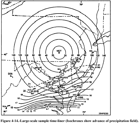 4.4.5.2 Plotting
and Analysis of the Time-Liner
4.4.5.2 Plotting
and Analysis of the Time-Liner